Directed Acyclic Graphs

A Directed Acyclic Graph is used to represent a Bayesian Network and like any other statistical graph, a DAG contains a set of nodes and links, where the links denote the relationship between the nodes.
A graphical model is a probabilistic model for which the conditional independence structure is encoded in a graph. In a graphical model, vertices (or nodes) represent random variables, and the edges encode conditional independence relations among the associated vertices. The graph characterizes the way in which the joint distribution factors into the product of many small components, each of which contains only a subset of variables.

Let X, Y and Z be random variables. X and Y are conditionally independent given Z, written X ㅛ Y | Z, if

p(x, y|z) = p(x|z) * p(y|z)

for all x, y and z.
Directed graphs are useful for representing conditional independence relations among variables. They can also be used to represent causal relationships
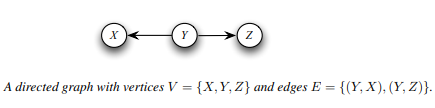
A directed graph G consists of a set of vertices V and an edge set E of ordered pairs of vertices. For our purposes, each vertex corresponds to a random variable. If (Y,X) ∊ E then there is an arrow pointing from Y to X.
If an arrow connects two variables X and Y (in either direction) we say that X and Y are adjacent. If there is an arrow from X to Y then X is a parent of Y and Y is a child of X. The set of all parents of X is denoted by πX or π(X). A directed path between two variables is a set of arrows all pointing in the same direction linking one variable to the other.

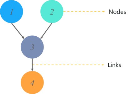
The nodes here represent random variables and the edges define the relationship between these variables. But what do these graphs model? What output can you get from a DAG?
A DAG models the uncertainty of an event occurring based on the Conditional Probability Distribution (CDP) of each random variable. A Conditional Probability Table (CPT) is used to represent the CPD of each variable in the network.
The first step is to build a Directed Acyclic Graph.
Consider the following example -
The graph has three nodes, each representing the door chosen by:
- The door selected by the Guest
- The door containing the prize (car)
- The door Monty chooses to open


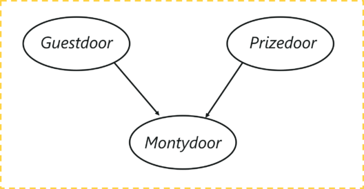
Let’s understand the dependencies here, the door selected by the guest and the door containing the car are completely random processes. However, the door Monty chooses to open is dependent on both the doors; the door selected by the guest, and the door the prize is behind. Monty has to choose in such a way that the door does not contain the prize and it cannot be the one chosen by the guest.
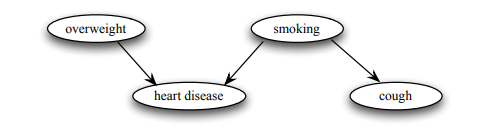
Consider the following DAG example, The probability function for the graph takes the following decomposition:
p(overweight,smoking, heart disease, cough) = p(overweight) * f(smoking) * p(heart-disease|overweight,smoking) * p(cough |smoking).

Naive Bayes Model

It is an instance of a much more general model commonly called the naive Bayes model. known as the Idiot Bayes model. The naive Bayes model assumes that instances fall into one of a number of mutually exclusive and exhaustive classes. Thus, we have a class variable C that takes on values in some set {c1, ..., ck}. In the reference of the [student problem], the class variable is the student’s intelligence I, and there are two classes of instances — students with high intelligence and students with low intelligence.

The model also includes some number of features X1,..Xn whose values are typically observed. The naive Bayes assumption is that the features are conditionally independent given the instance’s class. In other words, within each class of instances, the different properties can be determined independently. This model can be represented using the Bayesian Network.

The naive Bayes model, despite the strong assumptions that it makes, is often used in practice, because of its simplicity and the small number classification of parameters required. The model is generally used for classification — deciding, based on the values of the evidence variables for a given instance, the class to which the instance is most likely to belong.

Bayesian Network Model

Built on the same intuitions as the naive Bayes model by exploiting conditional independence properties of the distribution in order to allow a compact and natural representation.

Not restricted to representing distributions satisfying the strong independence assumptions implicit in the naive Bayes model allows us the flexibility to tailor our representation of the distribution to the independence properties that appear reasonable in the current setting.
Representation is a directed acyclic graph (DAG) G, whose nodes are the random variables in our domain and whose edges correspond to direct influence of one node on another.

Any graph G can be viewed in two very different ways:
1. As a data structure that provides the skeleton for representing a joint distribution compactly in a factorized way;
2. As a compact representation for a set of conditional independence assumptions about a distribution.

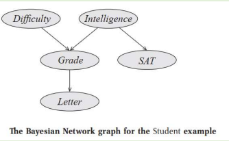
Student Example
Consider a student,
     - The student’s grade, in this case, depends not only on his intelligence but also on the difficulty of the course, represented by a random variable D whose domain is Val(D) = {easy, hard}
     - Students ask his professor for a recommendation letter. • The professor is absentminded and never remembers the names of her students. She can only look at his grade, and she writes her letter for him based on that information alone. • The quality of her letter is a random variable L, whose domain is Val(L) = {strong; weak}
     - The actual quality of the letter depends stochastically on the grade.
     - We therefore have five random variables in this domain:
           1. The student’s intelligence (I),
           2. The course difficulty (D),
           3. The grade (G),
           4. The student’s SAT score (S)
           5. The quality of the recommendation letter (L)

     - All of the variables except G are binary-valued, and G is ternary-valued.

A Bayesian network is represented using a directed graph whose nodes represent the random variables and whose edges represent direct influence of one variable on another.
We can view the graph as encoding a generative sampling process executed by nature, where the value for each variable is selected by nature using a distribution that depends only on its parents.
In other words, each variable is a stochastic function of its parents.